Transformer Study

개요

llama3.np 코드를 참고하여 토큰 입력부터 출력까지의 operation flow 를 정리한 문서

Operations

Make Encoder Input

텍스트 입력을 받아서 아래와 같은 절차를 통해 최종 인코더의 입력으로 들어갈 input 이 만들어진다.

• Text
  • Raw text input. (shape: (1, token_lengh))
• Tokenizing
  • Splitting text into tokens. (shape: (1, token_lengh))
• Token Encoding
  • Converting tokens to numerical IDs. (shape: (1, token_lengh))
• Token Embedding
  • Mapping token IDs to dense vectors. (shape: (1, token_lengh, dim))
• Positional Embedding
  • Adding positional information to embeddings. (shape: (1, token_lengh, dim))
• Final Representation
  • Combining token embeddings with positional embeddings.

Notation 정리

l : token 의 길이
d(dim): 하나의 token 이 가지는 vector 의 크기
vs(vocab size): vocab 크기
h (head): attention 에서 head 의 갯수

Transformer Architecture

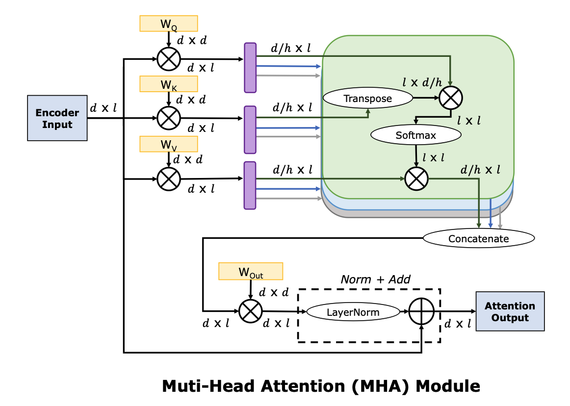
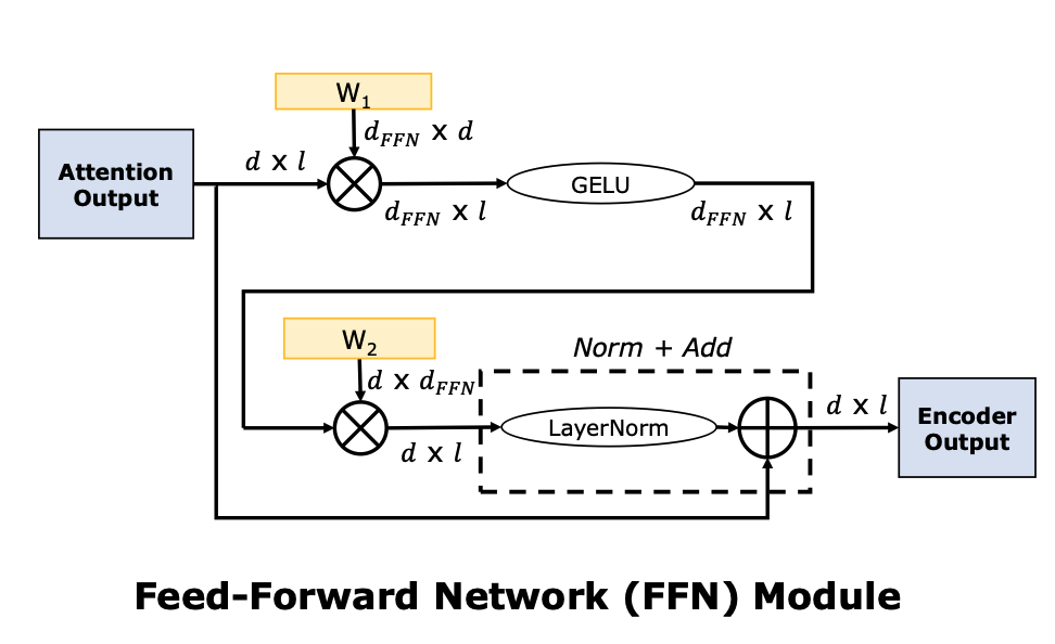
Full Stack Optimization of Transformer Inference: a Survey 논문에 나와있는 Encoder 의 attention 연산과 FFN 연산 도식도이다. LayerNorm 등의 위치는 LLM 모델마다 조금씩 차이가 있을 수 있으나 전체적인 flow 는 유사하다.

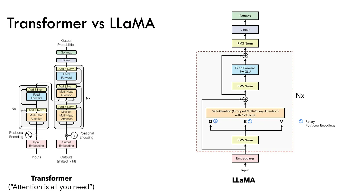
LLaMA Architecture

아래 그림은 llama 모델과 Attention is all you need 논문에서 소개되었던 Transformer 구조와의 다른 점을 보여준다. RMS Norm 이라는 개념과 Grouped Multi-Query Attention 그리고 KV Cache 라는 개념이 눈에 띄는데 각각에 대해서 자세히 살펴보도록 하자.

RMS Norm vs LayerNorm

TBU

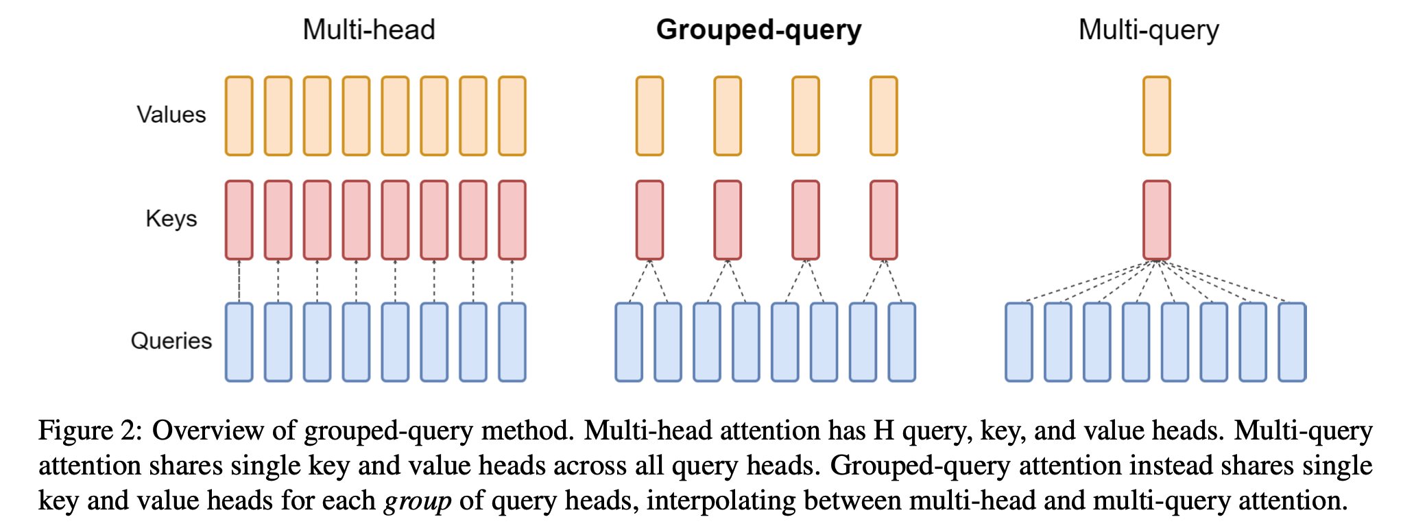
Grouped Multi-Query Attention

구글의 GQA 논문에서 처음 제시된 아이디어로 LLaMA 1 과 LLaMA 2 를 구분하는 큰 특징 중 하나라고 한다. 개념은 단순하다. K, Q, V 를 head 개수만큼 동일하게 쪼개서 연산하는게 MHA 이라면, GQA 는 Q 는 head 만큼 있고 K, V 는 head 의 약수 개로 이루어져 있는 건데 아래 그림을 참고하자.

이상하게 llama3.np 에서는 그냥 K, Q, V 모두 6개로 쪼개서 MHA 마냥 돌아가는게 디폴트 세팅값이긴 하다.

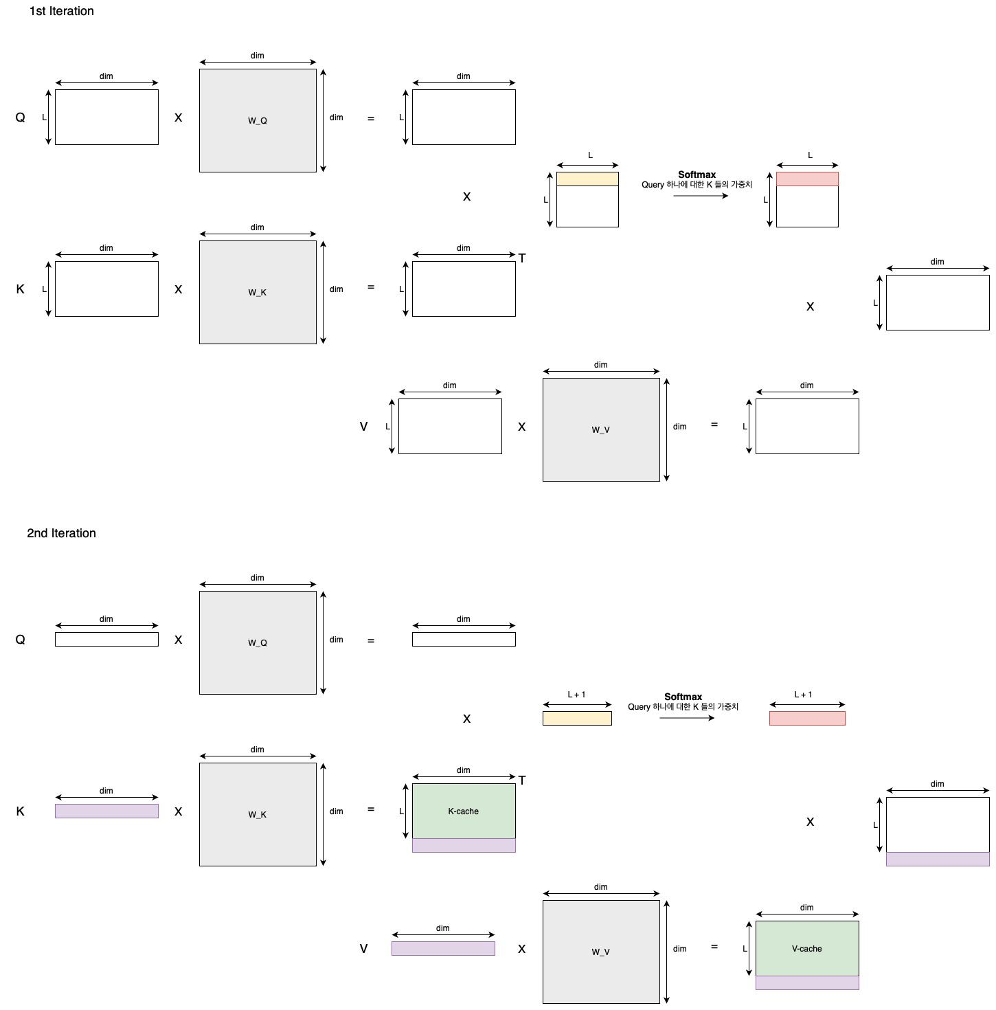
KV Cache

References

1. llama3.np 
2. Full Stack Optimization of Transformer Inference: a Survey
3. GQA